ViT：视觉Transformer开创者（论文+代码详解）

An Image is Worth 16x16 Words: Transformers for Image Recognition at Scale

Alexey Dosovitskiy (Google, Brain Team)

论文地址: ViT, arxiv

代码地址: timm-vision_transformer.py

动机：

是否CNN对于图像特征提取来说不是必须的？
NLP领域中，Transformer相关的Encoder和Decoder这一套框架是否可以代替CNN来完成图像领域的任务？

创新点：

将NLP领域的Transformer架构成功迁移到了CV领域，并且取得了和CNN相当的结果
不降低图像分辨率，将图像分成小的patch，加入位置编码后加入到网络中
实验表明，在超大数据集上训练，在常规数据集上Finetune后可以和CNN的SOTA结果相比较，所用计算资源也大大减少

实验参数：

结果汇总：

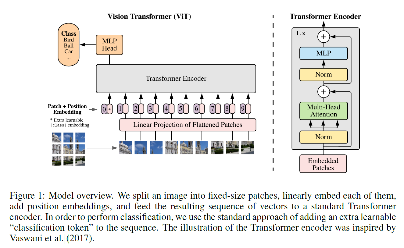
网络架构：

预处理（Embedding）：

Patch Embedding：将3维图像分patch，并且压缩到2维

操作分解：
1. 图像原始尺寸：\(B \times C \times H \times W\)
2. 按照patch块大小 \(P\) 切块，把patch内的像素放到channel维度 \((C*P^2) \times (H/P) \times (W/P)\)
3. 将channel维度线性映射到embedding dimension \(D\)，即变为 \(D \times (H/P) \times (W/P)\)
4. 将后两维flatten成一个维度 \(N\)，得到 \(D \times N\) 的张量
5. 将 \(D\) 和 \(N\) 所在的维度transpose，得到 \(N \times D\) 的张量，因为此时 \(D\) 中存的是patch的信息，这里就变成了feature map，而 \(N\) 则是patch的数量，相当于原始的channel
6. 对处理过后的张量做LN操作，即对每个feature map做归一化，LN共 \(2B \times N\) 个参数
7. 处理后的张量大小：\(B \times N \times D\)

代码解读：./timm/models/layers/patch_embed.py

class PatchEmbed(nn.Module):
    """ 2D Image to Patch Embedding
    """
    def __init__(self, img_size=224, patch_size=16, in_chans=3, embed_dim=768, norm_layer=None, flatten=True):
        super().__init__()
        img_size = to_2tuple(img_size)
        patch_size = to_2tuple(patch_size)
        self.img_size = img_size
        self.patch_size = patch_size
        self.grid_size = (img_size[0] // patch_size[0], img_size[1] // patch_size[1])
        self.num_patches = self.grid_size[0] * self.grid_size[1]
        self.flatten = flatten

        self.proj = nn.Conv2d(in_chans, embed_dim, kernel_size=patch_size, stride=patch_size) # 用卷积实现上述2、3步骤
        self.norm = norm_layer(embed_dim) if norm_layer else nn.Identity()

    def forward(self, x):
        B, C, H, W = x.shape
        _assert(H == self.img_size[0], f"Input image height ({H}) doesn't match model ({self.img_size[0]}).")
        _assert(W == self.img_size[1], f"Input image width ({W}) doesn't match model ({self.img_size[1]}).")
        x = self.proj(x) 
        if self.flatten:
            x = x.flatten(2).transpose(1, 2)  # 先把宽高维度flatten为N，然后将其与channel维度transpose # BCHW -> BNC 这里后者的C其实为embed_dim D
        x = self.norm(x) # 这里还有一个标准化层
        return x

Learnable Class Embedding

操作分解：（如果存在蒸馏，则同理加入蒸馏token）
1. 新建大小为 \(1 \times 1 \times D\) 维度的可训练的变量
2. .expand成 \(B \times 1 \times D\) 维度
3. 把patch embedding的结果与class embedding的结果在第一维上concat torch.cat()

代码解读：./timm/models/vision_transformer.py

class VisionTransformer(nn.Module):
    def __init__(...):
        # 只截取了相关的部分
        self.cls_token = nn.Parameter(torch.zeros(1, 1, embed_dim)) # 类别token 对应第1步
        self.dist_token = nn.Parameter(torch.zeros(1, 1, embed_dim)) if distilled else None # 蒸馏token
        self.pos_embed = nn.Parameter(torch.zeros(1, num_patches + self.num_tokens, embed_dim)) # PE Position Embedding
        self.pos_drop = nn.Dropout(p=drop_rate)
        
    def forward_features(self, x):
        x = self.patch_embed(x) # patch embedding
        cls_token = self.cls_token.expand(x.shape[0], -1, -1)  # 对应第2步
        if self.dist_token is None:
            x = torch.cat((cls_token, x), dim=1) # 对应第3步
        else:
            x = torch.cat((cls_token, self.dist_token.expand(x.shape[0], -1, -1), x), dim=1) # 如果蒸馏，则concat分类token、蒸馏token和patch token
        x = self.pos_drop(x + self.pos_embed)  # PE
        x = self.blocks(x)
        x = self.norm(x)
        if self.dist_token is None:
            return self.pre_logits(x[:, 0])
        else:
            return x[:, 0], x[:, 1]

Position Embedding
- 操作分解：
  1. 新建大小为 \(1 \times (N+1) \times D\) 维度的可训练的变量，其中 \(x\) 为额外加的token数量，通常为1或者2
  2. 将新建的变量+到embedding后的tensor（常量）上，不同batch共享同样的PE变量
- 代码解读：见上方Class Embedding

Transformer Encoder *L 重复L次

总览： \[ { z_0 = [x_{class};\ x_p^1E;\ x_p^2E;\ ···\ ;\ x_p^NE]+\ E_{pos},\ \ \ E \in R^{P^2C \times D},\ E_{pos} \in R^{(N+1) \times D} \ \ \ (1)\\\\\\ z'_l = MSA(LN(z_{l-1}))\ + \ z_{l-1}, \ \ \ l=1...L \ \ \ (2)\\\\ z_l = MLP(LN(z'_{l}))\ + \ z'_{l}, \ \ \ l=1...L \ \ \ (3)\\\\ y = LN(z^{0}_{L}) \ \ \ (4) } \]
- 操作分解：
\(z_0\) 为embedding后的结果，\(x_{class}\) 为分类token，\(x_p^i \in R^{1\times P^2C}\) 为图像分完patch后的向量，\(E\) 为线性变换矩阵，\(E_{pos}\) 为位置编码
1. 共有\(L\)个transformer结构，每个结构包含两个部分
2. 先做LN再做MSA，接一个shotcut
  1. 先做LN再做MLP，接一个shotcut
3. 将最后一个transformer的输出中的第0个patch取出来做LN后得到 \(y\) 用于分类

代码解读：

class Block(nn.Module):
  
    def __init__(self, dim, num_heads, mlp_ratio=4., qkv_bias=False, drop=0., attn_drop=0.,
                 drop_path=0., act_layer=nn.GELU, norm_layer=nn.LayerNorm):
        super().__init__()
        self.norm1 = norm_layer(dim)
        self.attn = Attention(dim, num_heads=num_heads, qkv_bias=qkv_bias, attn_drop=attn_drop, proj_drop=drop) # 这里对应Attention模块，其中Multi-head的数量就是 num_heads也就是注意力模块的数量
        # NOTE: drop path for stochastic depth, we shall see if this is better than dropout here
        self.drop_path = DropPath(drop_path) if drop_path > 0. else nn.Identity()
        self.norm2 = norm_layer(dim)
        mlp_hidden_dim = int(dim * mlp_ratio)
        self.mlp = Mlp(in_features=dim, hidden_features=mlp_hidden_dim, act_layer=act_layer, drop=drop) # 对应MLP模块，其中hidden_features就是指中间隐藏层降到的维数

    def forward(self, x):
        x = x + self.drop_path(self.attn(self.norm1(x))) # 对应上方的公式（2）
        x = x + self.drop_path(self.mlp(self.norm2(x))) # 对应上方的公式（3）
        return x

class VisionTransformer(nn.Module):       
    def __init__(...):
        # 只截取了相关代码
        dpr = [x.item() for x in torch.linspace(0, drop_path_rate, depth)]  # stochastic depth decay rule
        self.blocks = nn.Sequential(*[
            Block(dim=embed_dim, num_heads=num_heads, mlp_ratio=mlp_ratio, qkv_bias=qkv_bias, drop=drop_rate,attn_drop=attn_drop_rate, drop_path=dpr[i], norm_layer=norm_layer, act_layer=act_layer)
            for i in range(depth)]) # 用nn.Sequential(*[Block() for i in range(depth)])来完成transfermor结构重复depth次，depth=L
        self.norm = norm_layer(embed_dim)
        
    def forward_features(self, x):
        # 只截取部分代码
        x = self.blocks(x)
        x = self.norm(x)
        if self.dist_token is None:
            return self.pre_logits(x[:, 0])
        else:
            return x[:, 0], x[:, 1]

MSA(Multi-head Self Attention) 想了解一下head数量对于模型的影响！

Self Attention 机制：\(Attention(x) \ = \ Softmax(Q \times K^T/\sqrt{d}) \times V\)
- 为什么除以根号d？：防止 \(Q\times K^T\) 的数值过大，过 \(Softmax\) 时梯度消失
- \(Softmax(Q \times K^T/\sqrt{d})\) 整个相当于一个注意力矩阵，乘以原始图像 \(V\)
操作分解：
1. 将输入的 \(B\times N\times D\) 做线性变换为原来的三倍 \(B\times N\times 3*D\)
2. reshape成 \(B\times N\times 3 \times H \times (D/H)\)，其中 \(H\) 为Multi-head的数量，相当于把每个patch在分成H分，每一份都做不同的attention
3. permute重新排列为 \(3\times B\times H \times N \times (D/H)\)，然后unbind(0)得到 \(q,k,v\) 三个张量，大小为\(B\times H \times N \times (D/H)\)
4. 利用公式 \(Attention(x) \ = \ Softmax(q \times k^T/\sqrt{D/H}) \times v\) 计算注意力，中间会添加dropout防止过拟合
5. transpose(1,2).reshape(B, N, C)后将维度变换回了 \(B\times N\times D\)
6. 之后加一个全连接层，再接一个dropout层

代码解读：

class Attention(nn.Module):
    def __init__(self, dim, num_heads=8, qkv_bias=False, attn_drop=0., proj_drop=0.):
        super().__init__()
        assert dim % num_heads == 0, 'dim should be divisible by num_heads'
        self.num_heads = num_heads
        head_dim = dim // num_heads
        self.scale = head_dim ** -0.5

        self.qkv = nn.Linear(dim, dim * 3, bias=qkv_bias)
        self.attn_drop = nn.Dropout(attn_drop)
        self.proj = nn.Linear(dim, dim)
        self.proj_drop = nn.Dropout(proj_drop)

    def forward(self, x):
        B, N, C = x.shape
        qkv = self.qkv(x).reshape(B, N, 3, self.num_heads, C // self.num_heads).permute(2, 0, 3, 1, 4)
        q, k, v = qkv.unbind(0)   # make torchscript happy (cannot use tensor as tuple)

        attn = (q @ k.transpose(-2, -1)) * self.scale
        attn = attn.softmax(dim=-1)
        attn = self.attn_drop(attn)

        x = (attn @ v).transpose(1, 2).reshape(B, N, C)
        x = self.proj(x)
        x = self.proj_drop(x)
        return x

MLP(Multi Layer Processor)

操作分解：其实就是一个简单的降维再升维的操作，用全连接层实现
1. nn.Linear(in_dim, out_dim)全连接层将 \(B\times N\times D\) 变成 \(B\times N\times H\)，其中H为隐藏层维度
2. nn.Gelu激活函数层，增加非线性
3. nn.Dropout(p)随机丢弃一些点，不做正向传播和反向梯度更新
4. nn.Linear(in_dim, out_dim)全连接层将 \(B\times N\times H\) 变回 \(B\times N\times D\)，其中H为隐藏层维度
5. nn.Gelu激活函数层，增加非线性
6. nn.Dropout(p)随机丢弃一些点，不做正向传播和反向梯度更新

代码解读：

class Mlp(nn.Module):
    """ MLP as used in Vision Transformer, MLP-Mixer and related networks
    """
    def __init__(self, in_features, hidden_features=None, out_features=None, act_layer=nn.GELU, drop=0.):
        super().__init__()
        out_features = out_features or in_features
        hidden_features = hidden_features or in_features
        drop_probs = to_2tuple(drop)

        self.fc1 = nn.Linear(in_features, hidden_features)
        self.act = act_layer()
        self.drop1 = nn.Dropout(drop_probs[0])
        self.fc2 = nn.Linear(hidden_features, out_features)
        self.drop2 = nn.Dropout(drop_probs[1])

    def forward(self, x):
        x = self.fc1(x)
        x = self.act(x)
        x = self.drop1(x)
        x = self.fc2(x)
        x = self.drop2(x)
        return x

后处理（Classification）：

分类：

操作分解：
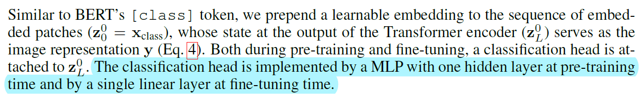
1. 对于Transformer的输出中class token对应的位置进行操作，先过一个MLP层，然后再过一个分类头后计算cross entropy loss
2. 这里预训练和微调时不太一样，微调时会把MLP层删掉，只留下分类头。这个操作应该是借鉴了自监督，因为自监督在预训练是没有类别信息，所以MLP后跟的是一个contrastive loss，用于计算输出与原始图像的loss

代码解读：

class VisionTransformer(nn.Module):       
    def __init__(...):
        # 只截取了相关代码
        # Representation layer
        if representation_size and not distilled:
            self.num_features = representation_size
            self.pre_logits = nn.Sequential(OrderedDict([  # 这里是预训练时的MLP层
                ('fc', nn.Linear(embed_dim, representation_size)),
                ('act', nn.Tanh())
            ]))
        else:
            self.pre_logits = nn.Identity()
        
    def forward_features(self, x):
        # 只截取部分代码
        if self.dist_token is None:
            return self.pre_logits(x[:, 0]) # 选取class token对应的区域进行分类
        else:
            return x[:, 0], x[:, 1]
        
    def forward(self, x):
        x = self.forward_features(x)
        if self.head_dist is not None:
            x, x_dist = self.head(x[0]), self.head_dist(x[1])  # x must be a tuple
            if self.training and not torch.jit.is_scripting():
                # during inference, return the average of both classifier predictions
                return x, x_dist
            else:
                return (x + x_dist) / 2
        else:
            x = self.head(x) # ViT不蒸馏直接分类
        return x